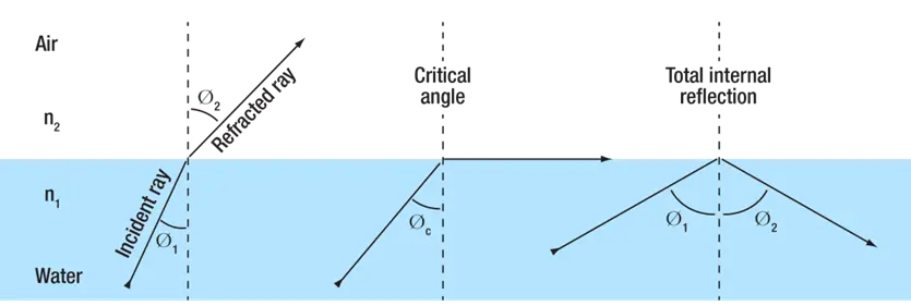
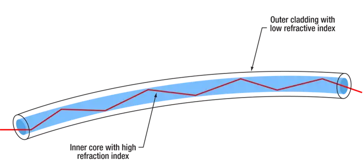
The basis of optical fiber is total internal reflection. As shown in the figure below, total internal reflection will occur when light is incident on the interface of high and low refractive materials at a shallow enough angle. Optical fibers use two types of glass with very small differences in refractive index. The central part is the core, and the outer part is called the cladding. The typical value of the core refractive index is 1.448 and the cladding is 1.444. The difference between the two refractive indexes is generally less than 1%, and even less than 0.5% for single-mode fiber. The core and cladding form a cylindrical waveguide, and light undergoes total internal reflection at the interface.
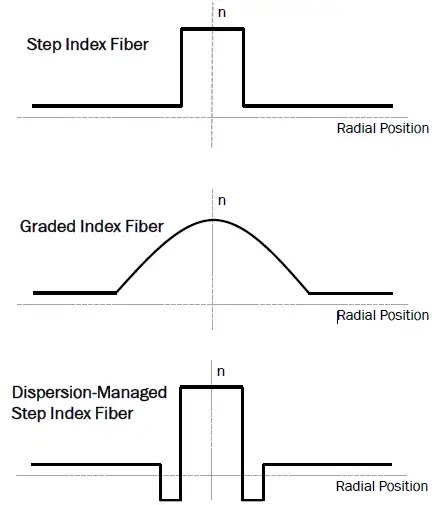
This article focuses on step-index fibers. Both the core and the cladding have a constant refractive index. The core is higher than the cladding, and the two refractive indexes change step by step. Some fibers use graded index or other more complex refractive index profiles, such as creating a low-refractive index depression around the core. Gradient index fibers are generally multimode fibers, which can achieve dispersion management purposes.
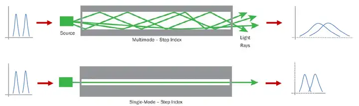
From a geometric optics perspective, light propagates along different paths in a multimode fiber using total internal reflection. From the perspective of wave optics, modes are equivalent to different paths that light takes. Some lights are in this mode and some lights are in other modes.

The fiber mode is a linear polarization mode, also called LP mode. This is because optical fibers are weak waveguides and are radially symmetrical. These LP modes are solutions of the complex electric field wave equation based on cylindrical coordinates. The LP mode has two indexes, the first is the azimuth index, and the second indicates how many solutions the first index has, so there are LP01, LP11, LP12 and other modes.
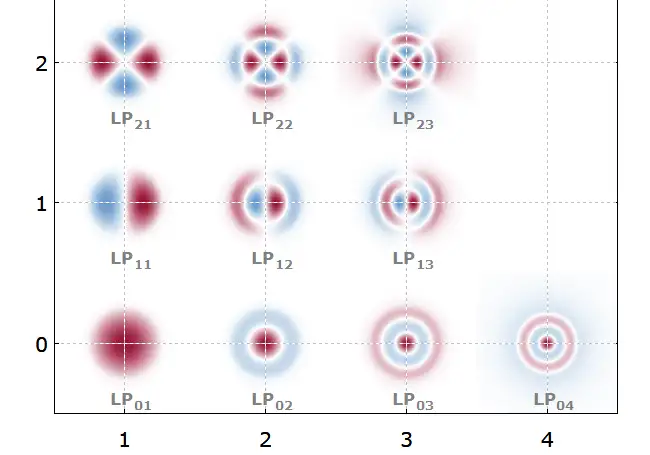
The first mode with an index greater than 1 is split, and may split from different angles such as up and down or left and right. Those are actually two mutually orthogonal modes, but here we treat them as one mode, and treat the orthogonal polarizations as the same mode. The image above shows a multimode fiber with very few modes, whereas a typical multimode fiber supports thousands of modes.
The following introduces the concept of single-mode fiber through a thought experiment. Assume that the core of a certain step-index multimode optical fiber is only 10 microns (actually it is usually tens or even hundreds of microns). We start with UV and gradually increase the wavelengths coupled into the fiber core. As the wavelength becomes longer, the fiber core becomes relatively smaller, so it can only accommodate fewer waves or modes, and the higher-order modes leak first and cannot be conducted by the fiber. At a certain wavelength, only two modes, LP11 and LP01, will be left. As the wavelength continues to become longer, the second mode LP11 and the first mode LP01 are also cut off successively. At this time, the optical fiber cannot conduct any light.
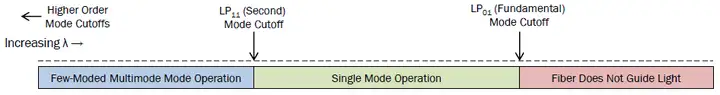
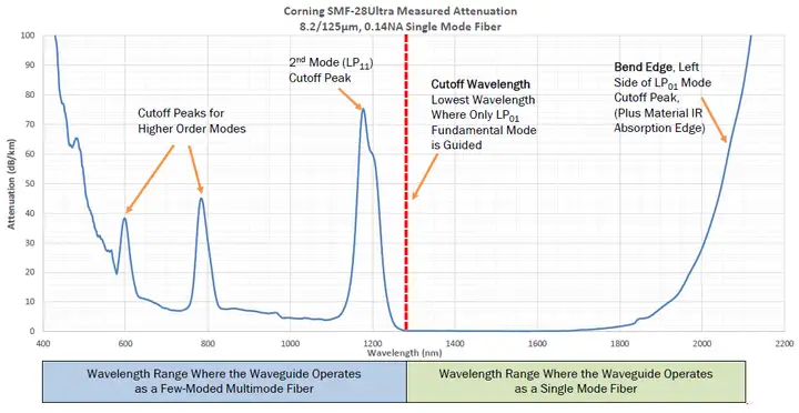
Therefore, within the wavelength range between the second mode cutoff and the first mode cutoff, the optical fiber can only conduct the LP01 mode, also called the fundamental mode. This range is the single-mode wavelength range. In the figure below, the short-wavelength blue area represents the multimode operating range of very few modes, the green area represents the single-mode operating range, and the long-wavelength red area exceeds the cutoff of the LP01 mode, at which point the fiber cannot conduct any light.
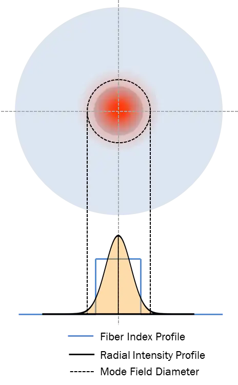
If you look at the cross-sectional profile of a single-mode fiber, the fundamental mode is slightly larger than the core and slightly into the cladding. The fundamental mode intensity profile is close to a Gaussian shape, and the 1/e² diameter of the fundamental mode intensity is also called the mode field diameter (MFD). When performing fiber coupling, the mode field diameter can be used as the effective core size. Because the mode field diameter is larger than the fiber core, although the highest light intensity is at the center of the fiber core, there is a large intensity area outside the fiber core, so about 45% of the optical power propagates in the cladding instead of the core.
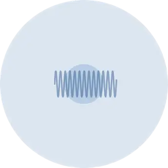
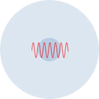
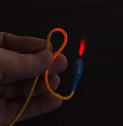
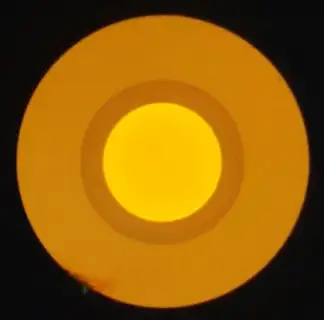
The following two pictures are the output spots of single-mode and multi-mode optical fibers in the far field respectively. The single-mode light spot is close to Gaussian shape, while the multi-mode light spot looks more messy. Assuming that coherent laser light is coupled into a multimode fiber, all modes interfere constructively or destructively in the larger fiber core, thus forming speckles. However, the output of single-mode fiber has no speckle effect, but an almost perfect Gaussian shape, and has nothing to do with coupling conditions. Single-mode fiber can also be used for mode filtering, coupling mixed-mode beams into single-mode fiber, and the fiber will output a beautiful Gaussian beam.


Single-mode fiber is bend insensitive, that is, it is very little affected by bending. When a multimode fiber is bent, the optical power distribution between different modes will change, and the optical power generally shifts to higher-order modes. Higher order modes have high losses, so bending of multimode fiber increases the loss. In single-mode fiber, the propagation of the fundamental mode is relatively unaffected by bending, and the output pattern does not change due to bending.
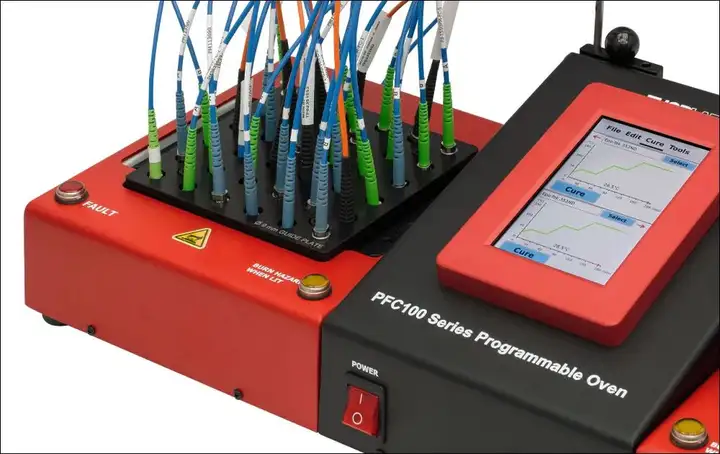
It is worth mentioning that regarding the image comparison between single-mode and multi-mode output patterns, the previous video fully records the experimental process starting at 18:30. In addition, fiber optic patch cords were used in the experiment. In order to achieve high-efficiency automation of fiber jumper production, Thorlabs has recently launched Vytran connector production equipment : CO2 laser fiber cutting machine and fiber connector curing oven. The former is used to cut epoxy resin beads, and the latter is used to cure epoxy resin. The actual equipment and usage details are as follows.

The superior performance of single-mode fiber, of course, comes at a price. For optical fibers to be single-mode, the fiber core must be small. In order to conduct only the fundamental mode, the single-mode core is much smaller than the multi-mode core. This means that it is more difficult to achieve high coupling efficiency when coupling with single-mode fibers. Not only must the coupling components have very accurate mechanical positioning freedom, but also the fibers, beams and lenses must be precisely aligned. When two single-mode optical fibers are mechanically spliced or otherwise interconnected, the loss can easily become high if the component tolerances are not strict enough. Imagine that for a 9 μm core, in order to achieve high coupling efficiency, there cannot be an offset error of several microns between the two fibers, and the input beam must be a good Gaussian beam.

The next property of the fundamental mode is related to fiber optic communications. Single-mode optical fibers are widely used in global communications because they have no inter-modal dispersion. With single-mode fiber, light can only travel in one mode and along one path. Multimode fiber has different modes and different effective path lengths, which cause time broadening when transmitting signal pulses, making them indistinguishable to detectors. Relatively speaking, single-mode optical fiber does not have the above problems, so it can achieve the highest data transmission speed.
The attenuation of single-mode fiber is generally much lower than that of multi-mode fiber. One of the basic reasons is that light can only be transmitted in the LP01 fundamental mode, and power cannot be transferred to high-loss high-order modes. In addition, due to continuous optimization of production and design, single-mode optical fiber continues to set world records for ultra-low attenuation.
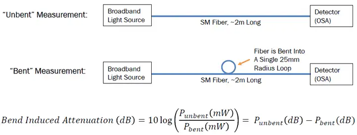
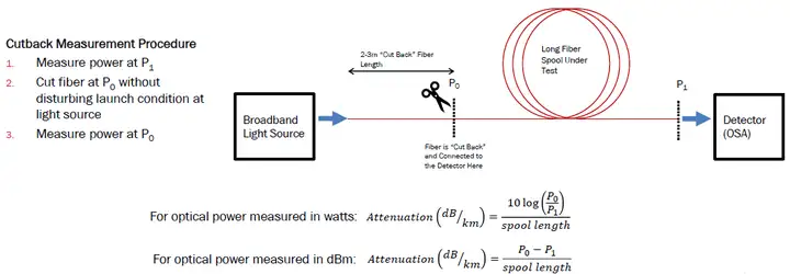
In order to study the mode properties of single-mode fiber, we make a circle with a certain radius in the middle of the fiber, and compare the power of straight fiber and curved fiber to obtain the attenuation curve. The measurement schematic diagram and calculation formula are as follows. We couple a broadband light source and measure the power distribution in a wide wavelength range through an optical spectrum analyzer (OSA).
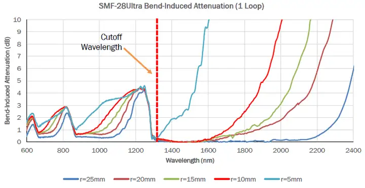
Taking a typical SMF-28 Ultra fiber as an example, the actual measured bend-induced attenuation curve is as follows. There are several peaks on the curve appearing at certain wavelengths. We explain the causes of these peaks based on the basic meaning of single-mode fiber. When the fiber is bent, if there are two modes, some power is transferred to the higher-order mode, and the higher-order mode has higher bending loss. If a mode is near a wavelength where it cannot be carried by the fiber, the mode will have high bend-induced attenuation.
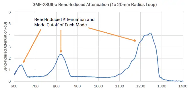
First look at this peak near 800 nm. There are several propagation modes in the fiber at this time. When the wavelength increases from around 800 nm, the bend-induced attenuation increases. This is because a certain mode is about to be unable to conduct, so the bend-induced loss is very high. As the wavelength continues to increase, that mode disappears from the fiber, that is, the fiber no longer conducts that mode, so the attenuation returns to baseline levels.
The wavelength corresponding to a mode that experiences high attenuation and then disappears is called the cutoff wavelength of this mode. The three peaks of the curve correspond to the three blocked modes. As the wavelength becomes longer, the total number of modes becomes smaller, so the power contribution of each mode becomes higher, resulting in higher and higher peaks.
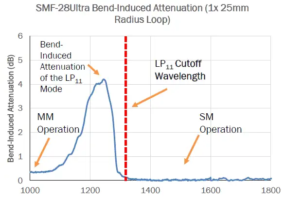
The rightmost part of the above curve is also worth noting. The attenuation here seems to be almost zero, so we need to introduce the concept of cutoff wavelength. As shown in the figure below, the cut-off wavelength is the wavelength corresponding to when the second mode begins to be unable to be transmitted by the optical fiber. The optical fiber then enters the single-mode operating wavelength range and can only conduct the LP01 mode and is insensitive to bending.
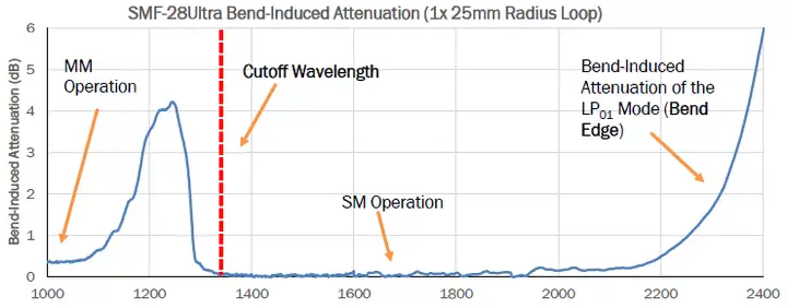
Let's keep increasing the wavelength and see what happens. Regarding the bend-induced attenuation curve in the figure below, in the single-mode wavelength range, the optical fiber has basically no bend-induced attenuation, but there is another peak starting to rise on the right. After reaching such a long wavelength, the conduction of the LP01 fundamental mode also becomes weaker, and high bending losses begin to occur. This is actually the left side of the peak, but because the fiber cannot guide light to the right, we cannot measure the other side. This is also the beginning of the LP01 fundamental mode cutoff wavelength peak, which is called the bending edge.
The previous bending-induced attenuation measurement used a ring with a radius of 25 mm. The following compares the attenuation curves under different ring radii, and adds the measurement data at 20, 15, 10 and 5 mm radii. The smaller the ring radius, the sooner the second mode becomes high loss, that is, it occurs at a shorter wavelength. But the cut-off wavelength remains constant (dashed red line) regardless of the size of the ring. In addition, the smaller the bending radius, the narrower the single-mode range. Therefore, if the fiber is not bent, the fiber can be used further toward the infrared region.
Finally, spectral attenuation is introduced. We are going to couple the light into several kilometers of fiber wound on a spool and measure the power versus wavelength. This test also uses a broadband light source and an optical spectrum analyzer (OSA). Then without changing the coupling conditions, cut the optical fiber a few meters away from the coupling point, and connect the OSA to the P0 point to rescan and measure the relationship between power and wavelength. By comparing the measurement results of P1 and P0 you can know how much light is lost between the two points.
This method is called the cutback method, and it is the standard method for measuring spool attenuation. The attenuation per meter or average attenuation can be obtained by dividing the power difference at two points by the fiber length, but it is generally expressed in dB/km. Below is the measurement diagram and calculation formula.
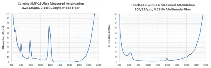
The figure below shows the spectral attenuation curve of SMF-28 single-mode fiber. There are also cutoff peaks for different modes on this curve, and you can see the cutoff, single-mode operating range and bending edge of the LP11 mode. On the far right side of the curve, in addition to the effect of the curved edge, there is also material absorption, as the light passes through several kilometers of glass fiber. When the wavelength is close to 2 μm, the crystal lattice absorbs photons to generate vibration energy due to multi-phonon absorption. The attenuation also starts to increase as we approach the UV region on the left side of the curve. This is also because the material absorbs, but not vibrational energy, electrons are excited to higher energy levels, so electron absorption is responsible for the rise in UV attenuation.
Different from single-mode fiber, the attenuation curve of multi-mode fiber does not have a mode cutoff peak, but there are several absorption peaks with completely different properties, and the lowest attenuation is far from the level of single-mode fiber. However, the infrared and ultraviolet absorption edges from the material are similar on both sides of the curve.
Taking step-index single-mode fiber design as an example, the two variables we can control are core diameter and fiber NA. Shown below are two optical fiber cross-sections taken through a microscope. Although the core size is very different and the NA is different, both fibers have the same cutoff wavelength. By choosing two different sets of parameters, the light guiding performance is different, but the combination of the two can achieve the same cut-off wavelength, so these are two different ways to design single-mode fiber.


NA (numerical aperture) is related to the difference in refractive index between the core and cladding. The higher the NA, the
![Singi Cable[Email: singi100@singi.com]](/u_file/2303/photo/11c1fa1eb8.jpg)

